Image Analysis/Processing
Diffraction patterns analysis is essentially specialized image processing. This tutorial will show some of the image processing and analysis techniques that are part of the scikit-ued.
Note
Use scikit-ued in combination with npstreams to process electron diffraction data in parallel.
Reading Images
Diffraction patterns can come in a variety of exotic file formats. Scikit-ued has built-in support for the following file formats:
Gatan’s closed source DM3 and DM4 (*.dm3, *.dm4);
Merlin Image Binary (*.mib);
TIFF images (*.tif, *.tiff);
All other file formats supported by scikit-image.
The diffread() function will transparently distinguish between those formats and dispatch to the right functions.
.. _automatic_mask_generation:
Automatic generation of a mask as needed for the autocenter() function
Automatic mask generation
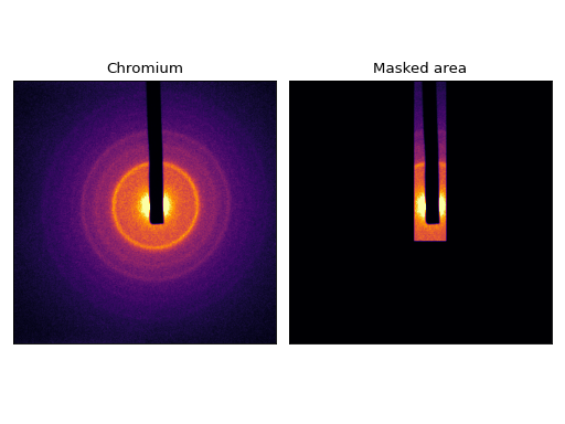
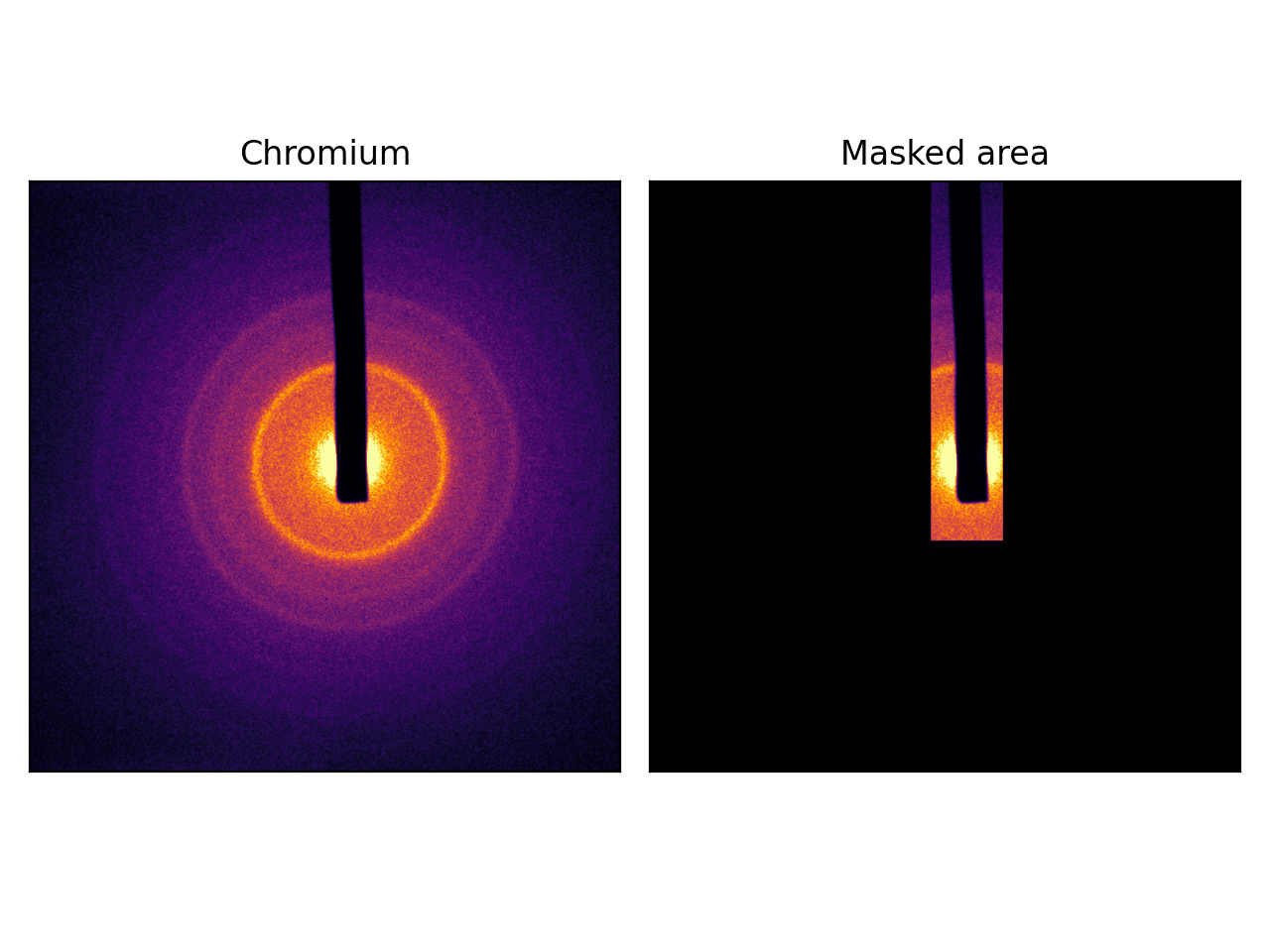
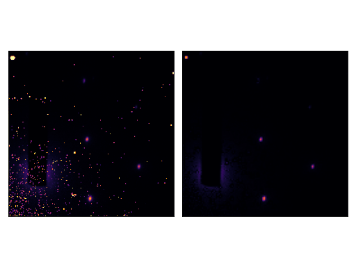
A mask can be used for the :func: autocenter function to exclude the beam stopper from the analysis and only keep valuable information. Such a mask can automatically be generated using this function; given a diffraction pattern, the mask will be created to block the darkest regions of the image (default blocks about 10% of the darker values). Here is an example:
(Source code, png, hires.png, pdf)

Automatic center-finding
Many analyses involving diffraction patterns require the knowledge of the center. For this purpose, scikit-ued
provides autocenter(). It can be used trivially as follows:
>>> from skued import diffread, autocenter
>>> import numpy as np
>>>
>>> im = diffread('docs/tutorials/data/Cr_1.tif')
>>>
>>> # Invalid pixels are masked with a False
>>> mask = np.ones_like(im, dtype = bool)
>>> mask[0:1250, 975:1225] = False
>>>
>>> center = autocenter(im, mask=mask)
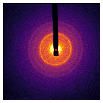
Let’s take a look at the result. The center is shown with a red dot:
(Source code, png, hires.png, pdf)

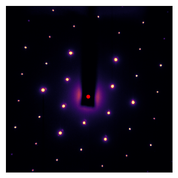
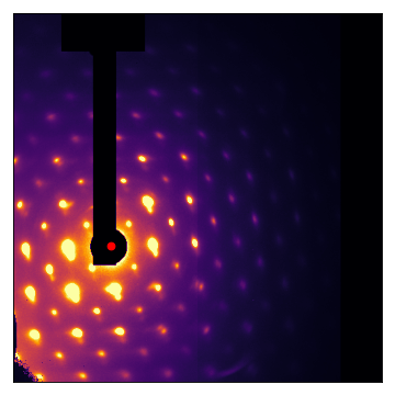
We can do the same with single-crystal diffraction patterns:
>>> from skued import diffread, autocenter
>>> import numpy as np
>>>
>>> im = diffread('docs/tutorials/data/graphite.tif')
>>> mask = diffread('docs/tutorials/data/graphite_mask.tif').astype(bool)
>>>
>>> center = autocenter(im, mask=mask)
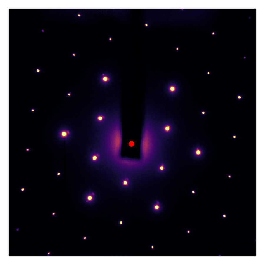
Let’s take a look at the result. The center is shown with a red dot:
(Source code, png, hires.png, pdf)
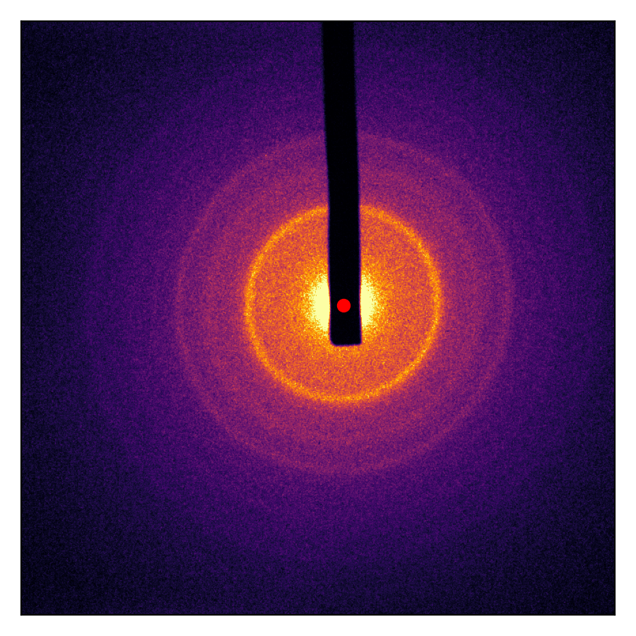
autocenter() also works with images that are very off-center and display large Ewald-sphere walkoff:
(Source code, png, hires.png, pdf)
It’s worth emphasizing that apart from the mask, there are no parameters to play with; autocenter() is as automatic as it can be!
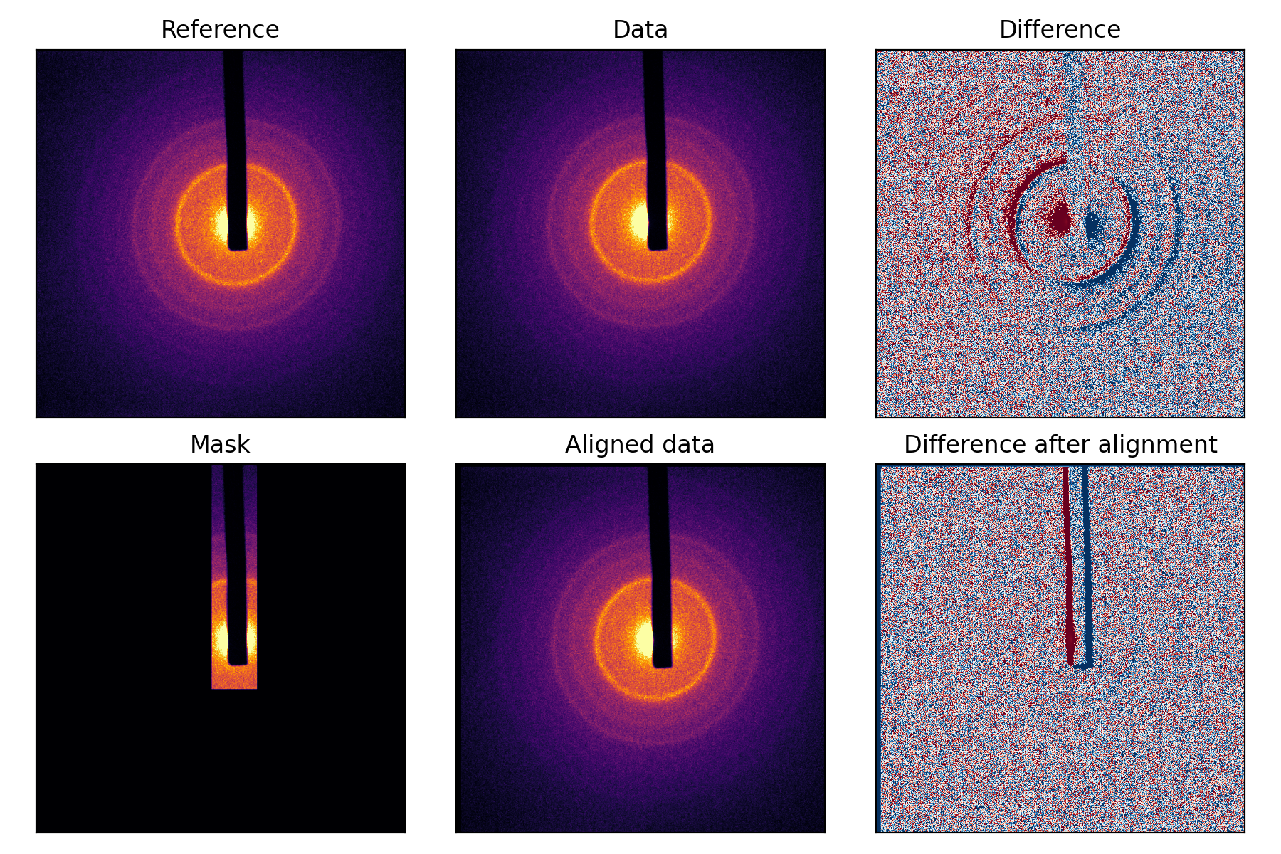
Diffraction pattern alignment
Diffraction patterns can drift over a period of a few minutes, and for reliable data synthesis it is important to align patterns to a reference.
Diffraction patterns all have a fixed feature: the position of the beam-block. Therefore, some pixels in each diffraction pattern must be ignored in the computation of the cross-correlation.
Setting the ‘invalid pixels’ to 0 will not work, at those will correlate with the invalid pixels from the reference. One must use the masked normalized cross-correlation.
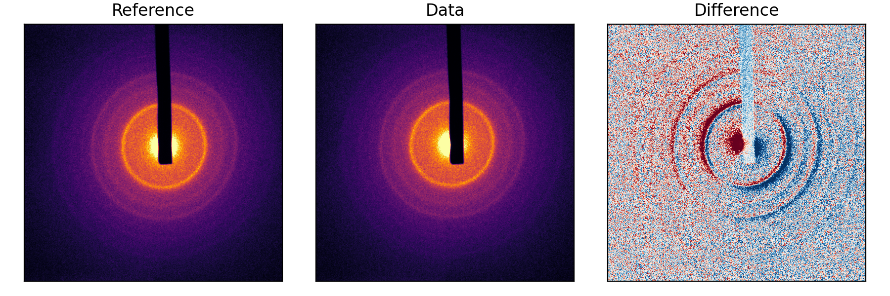
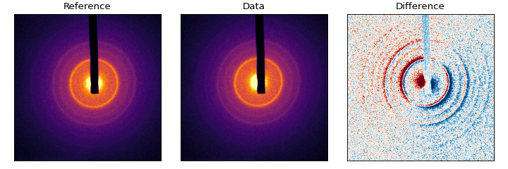
All of this is taken care of with the align() function. Let’s look at some polycrystalline Chromium:
(Source code, png, hires.png, pdf)

From the difference pattern, we can see that the ‘Data’ pattern is shifted from ‘Reference’ quite a bit, but the beamblock has not moved. To determine the exact shift, we need to use a mask that obscures the beam-block and main beam:
>>> from skued import diffread, align
>>> import numpy as np
>>>
>>> ref = diffread('docs/tutorials/data/Cr_1.tif')
>>> im = diffread('docs/tutorials/data/Cr_2.tif')
>>>
>>> # Invalid pixels are masked with a False
>>> mask = np.ones_like(ref, dtype = bool)
>>> mask[0:1250, 975:1225] = False
>>>
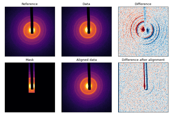
>>> aligned = align(image=im, reference=ref, mask=mask)
Let’s look at the difference:
(Source code, png, hires.png, pdf)

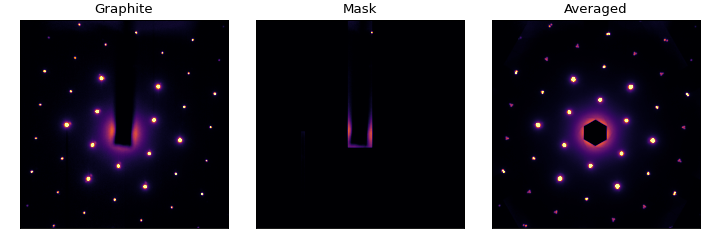
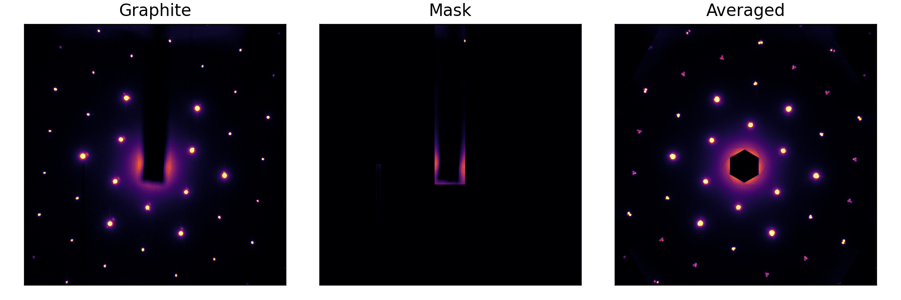
Image processing involving symmetry
Rotational symmetry
Diffraction patterns exhibit rotational symmetry based on the crystal structure. We can
take advantage of such symmetry to correct images in case of artifacts or defects. A useful
routine is nfold(), which averages portions of a diffraction pattern with itself based on
rotational symmetry.
(Source code, png, hires.png, pdf)

To use nfold(), all you need to know is the center of the diffraction pattern:
>>> from skued import nfold, diffread
    >>>
>>> im = diffread('docs/tutorials/data/graphite.tif')
>>> av = nfold(im, mod = 6, center = (1024, 1024))    # mask is optional
Pixel Masks
Image data can be rejected on a per-pixel basis by using pixel masks. These masks are represented
by boolean arrays that evaluate to Falose on invalid pixels, and True otherwise
scikit-ued offers some functions related to creation and manipulation of pixel masks.
Creation of a pixel mask
A pixel mask can be created from a set of images sharing the same properties. For example, diffraction patterns before photoexcitation (i.e. dark runs) form a set of images that should be identical.
Let’s imaging a set of such images with filenames dark_run_*.tif. We can create a pixel mask with the mask_from_collection():
>>> from glob import iglob
>>> from skued import mask_from_collection, diffread
    >>>
>>> dark_runs = map(diffread, iglob('dark_run_*.tif'))
>>> mask = mask_from_collection(dark_runs)
In the above example, pixel values outside opf the [0, 30000] range will be marked as invalid (default behaviour). Moreover, the per-pixel standard deviation over the image set is computed; pixels that fluctuate too much are also rejected.
Note that since mask_from_collection() uses npstreams under the hood, the collection of files used to compute the
mask can be huge, much larger than available memory.
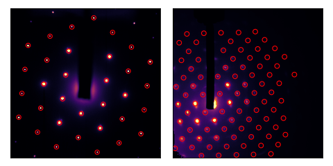
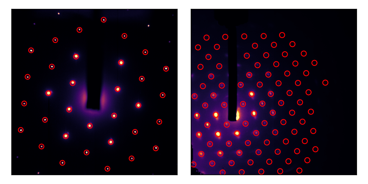
Finding Bragg peaks
The first step in any single-crystal indexing routine is to find Bragg peaks. To this end, the
bragg_peaks() function can be used as follows:
>>> from skued import diffread, bragg_peaks
>>>
>>> im = diffread('docs/tutorials/data/graphite.tif')
>>> mask = diffread('docs/tutorials/data/graphite_mask.tif').astype(bool)
>>>
>>> peaks = bragg_peaks(im, mask=mask)
We can plot the result:
(Source code, png, hires.png, pdf)
How cool is that!
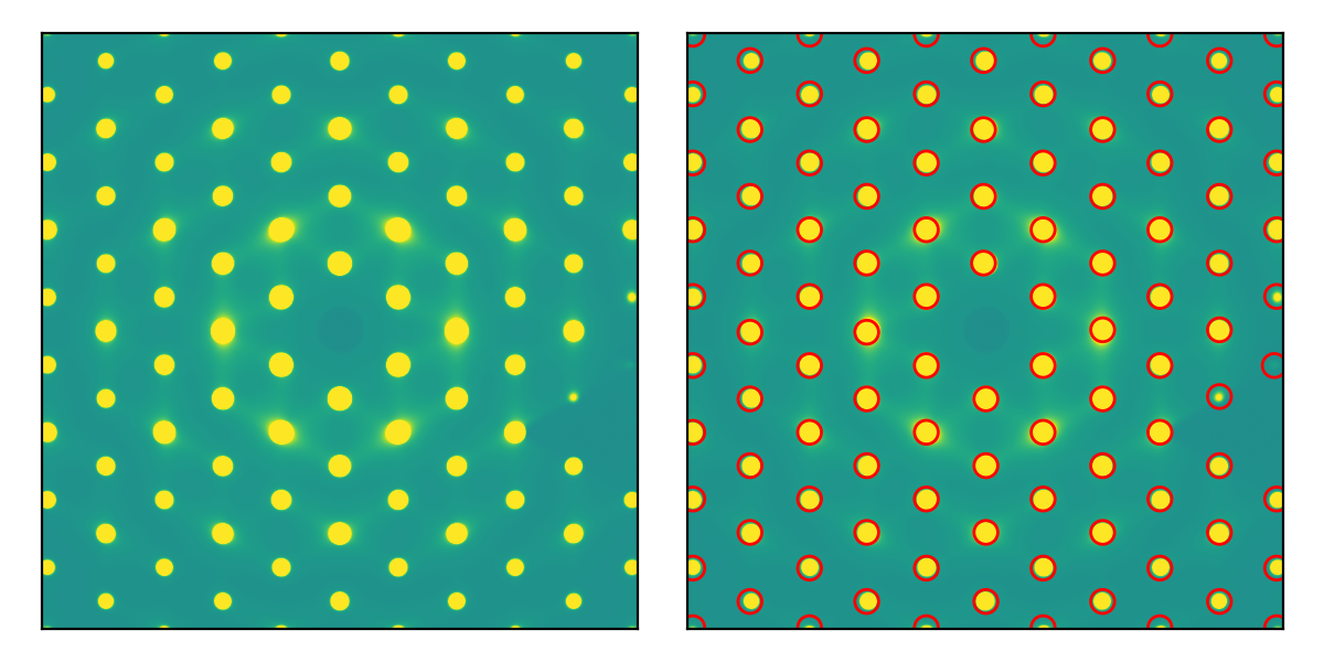
We can also use the method of 2D peak topological persistence to find Bragg peaks. Using the
bragg_peaks_persistence() function, we determine the peaks via:
>>> from skued import diffread, bragg_peaks_persistence
>>>
>>> im = diffread('docs/tutorials/data/ab_initio_monolayer_mos2.tif')
>>>
>>> peaks, bd, bd_indices, persistence = bragg_peaks_persistence(im, prominence=0.1)
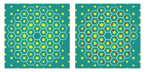
We plot the results. The left plot shows that the standard bragg_peaks() finds no peaks,
while bragg_peaks_persistence() finds all of them, given on the right :
(Source code, png, hires.png, pdf)
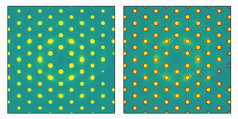
Finding Brillouin zones
We can also determine Brillouin zones based on the location of Bragg peaks.
For normal incidence diffraction, such patterns are regular polygons for
simple crystal structures, but for tilted-incidence diffraction or macromolecules,
the geometry becomes unclear, necessitating a different approach. The Brillouin zone,
the Wigner-Seitz unit cell in reciprocal space, is also the Voronoi regions determined
by the Bragg peak locations. This functionality is implemented in this package
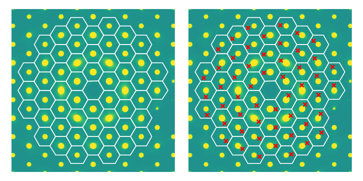
by the class brillouin_zones.
>>> from skued import diffread, autocenter, bragg_peaks_persistence, brillouin_zones
>>>
>>> im = diffread('docs/tutorials/data/ab_initio_monolayer_mos2.tif')
>>>
>>> peaks, bd, bd_indices, persistence = bragg_peaks_persistence(im, prominence=0.1)
>>> center = np.array([im.shape[0]//2, im.shape[1]//2])
>>> BZ = brillouin_zones(im, mask=np.ones(im.shape), peaks=peaks.astype(int), center=center.astype(int))
We can even determine equivalent scattering vectors at all visible
Brillouin zones via the getEquivalentScatteringVectors() method, useful for averaging the signal at a given reduced wavevector
for low SNR single-crystal datasets, visualized explicitly on the right.
(Source code, png, hires.png, pdf)

Image analysis on polycrystalline diffraction patterns
Angular average
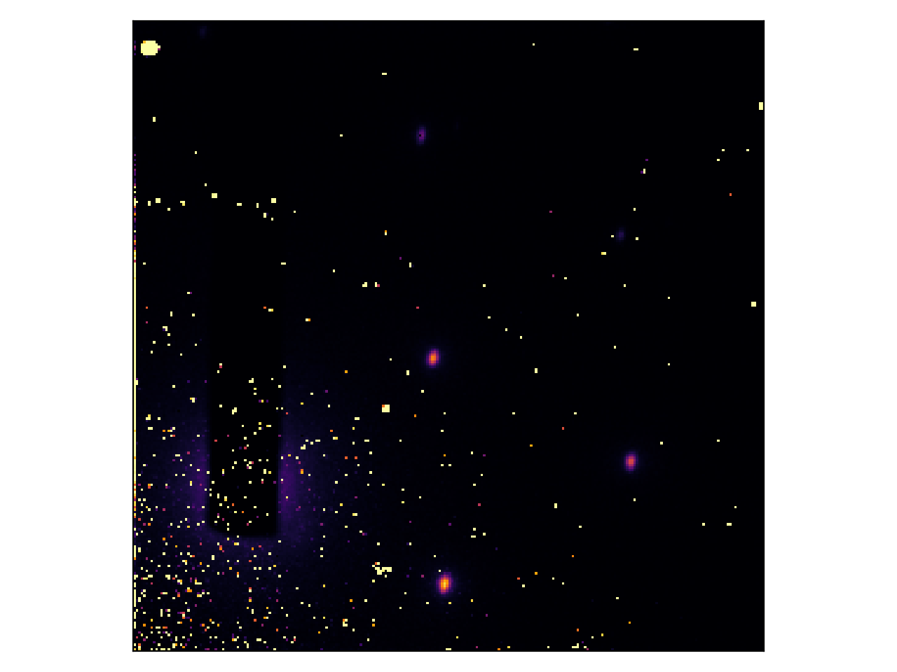
First, let’s load an image:
>>> import numpy as np
>>> import matplotlib.pyplot as plt
>>> from skued import diffread, autocenter
>>>
>>> image = diffread("docs/tutorials/data/Cr_1.tif")
>>>
>>> mask = np.ones_like(image, dtype = bool)
>>> mask[0:1250, 975:1225] = False
>>>
>>> plt.imshow(image)
>>> plt.show()
(Source code, png, hires.png, pdf)
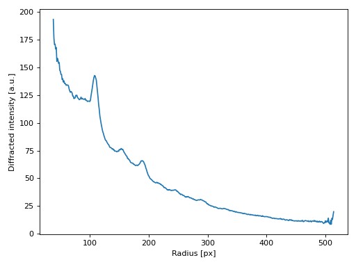
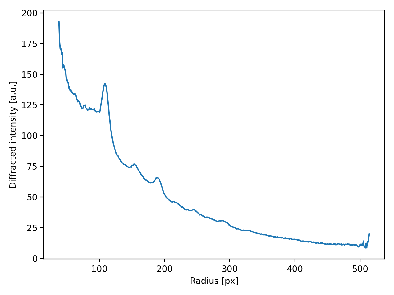
… and we can easily compute an angular average:
>>> from skued import azimuthal_average, autocenter
>>>
>>> yc, xc = autocenter(image, mask=mask)
>>> radius, intensity = azimuthal_average(image, (xc, yc), mask=mask)
>>>
>>> plt.plot(radius, intensity)
(Source code, png, hires.png, pdf)
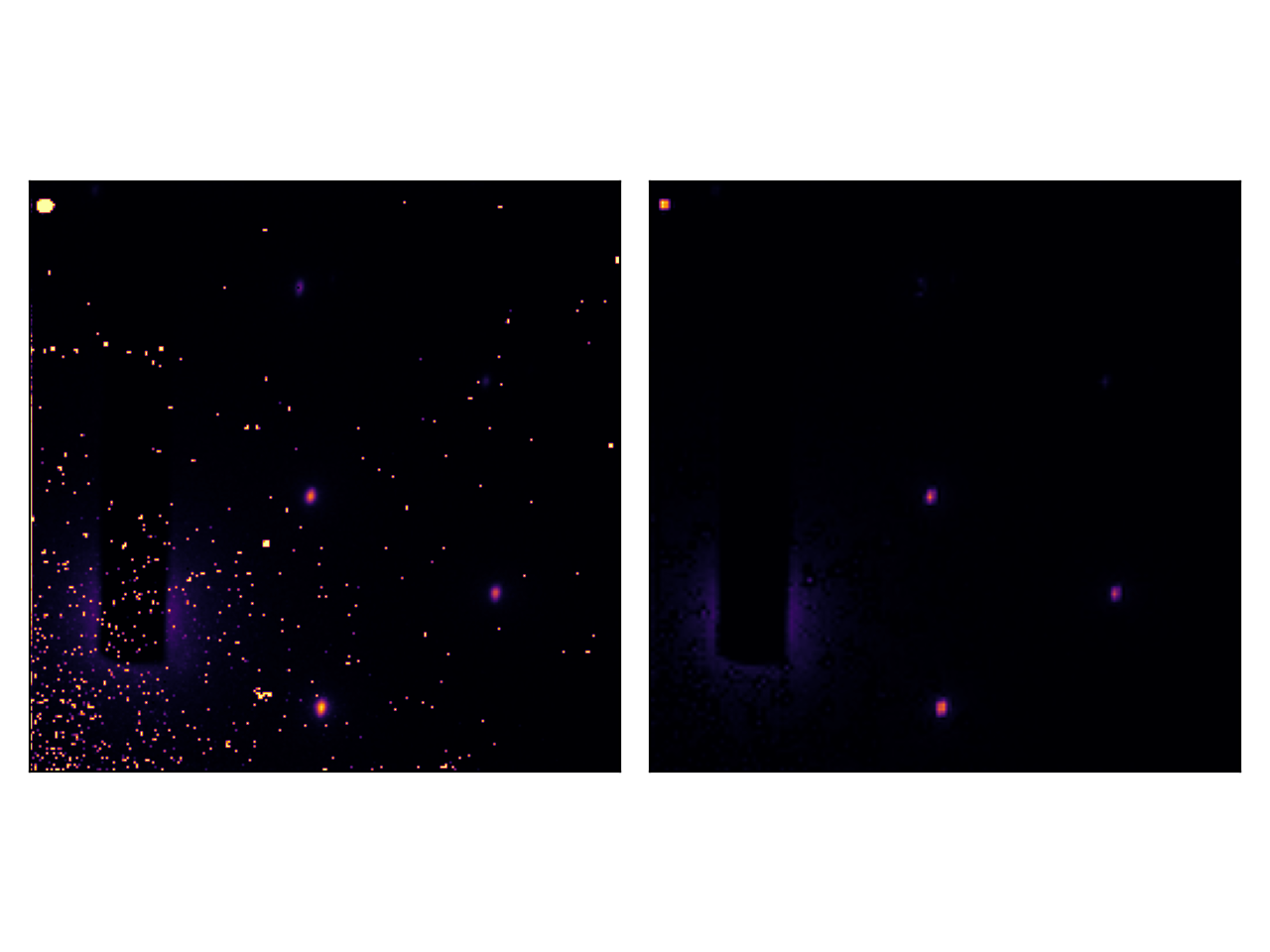
Bonus : Removing Hot Spots
An interesting use-case of baseline-removal (described in Baseline-determination) is the removal of hot spots from images.
Consider the following diffraction pattern:
(Source code, png, hires.png, pdf)
We can consider the image without hotspots as the baseline of the image with hotspots :
>>> from skued import diffread, baseline_dwt
>>>
>>> im = diffread('docs/tutorials/data/hotspots.tif')
>>> denoised = baseline_dwt(im, max_iter = 250, level = 1, wavelet = 'sym2', axis = (0, 1))
The result is plotted below:
(Source code, png, hires.png, pdf)

Try different combinations of wavelets, levels, and number of iterations (max_iter).
Notice that the baseline-removal function used in the case of an image is baseline_dwt(), which works on 2D arrays.
The same is not possible with baseline_dt(), which only works on 1D arrays at this time.