Time-series analysis
Time-resolved diffraction measurements reduce down to a (large) series of time-series. Exploring those time-series reveal the dynamics captured by experiments. This tutorial will go over some of the functions that help this data exploration.
Fitting
Time-resolved experiments are powerful tools because they can be used to distinguish separate processes by their characteristic time-scales. Therefore, extracting time-constants from dynamics is an important tool.
skued exports some curves that make it much easier to fit to scattering time-series:
>>> import numpy as np
>>> import skued
>>> from scipy.optimize import curve_fit
>>>
>>> # Load data from file first
>>> # 2 x N array:
>>> #   first row is time-delay
>>> #   second row is diffracted intensity
>>> block = np.load('docs/tutorials/data/tseries1.npy')
>>> time, intensity = block[0, :], block[1, :]
>>>
>>> # Compute initial guesses for this curve (optional)
>>> initial_guesses = (0,                                   # time-zero
...                    intensity.max() - intensity.min(),   # amplitude
...                    1,                                   # time-constant
...                    intensity.min())                     # offset
>>>
>>> params, pcov = curve_fit(skued.exponential, time, intensity,
...                          p0 = initial_guesses)
>>>
>>> tzero, amplitude, tconst, offset = params
>>> best_fit_curve = skued.exponential(time, *params)
>>> # Equivalent:
>>> #   best_fit_curve = skued.exponential(time, tzero, amplitude, tconst, offset)
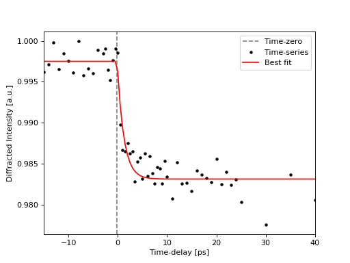
We can plot the result:
(Source code, png, hires.png, pdf)

Taking into account the IRF
No fitting of time-resolved data is complete without taking into account the instrument response function,
or IRF. To help with this, scikit-ued provides the with_irf() decorator factory. It can be used as follows:
>>> from skued import exponential, with_irf
>>>
>>> # If the data is recorded in picoseconds, then the following
>>> # applies a Gaussian IRF with a full-width at half-max of 150fs (0.15 picoseconds)
>>> @with_irf(0.150)
... def exponential_with_irf(time, *args, **kwargs):
...     return exponential(time, *args, **kwargs)
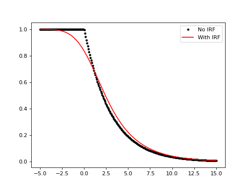
Let’s see what with_irf() in action:
(Source code, png, hires.png, pdf)

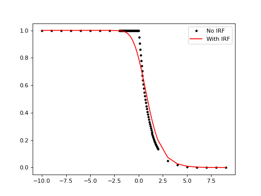
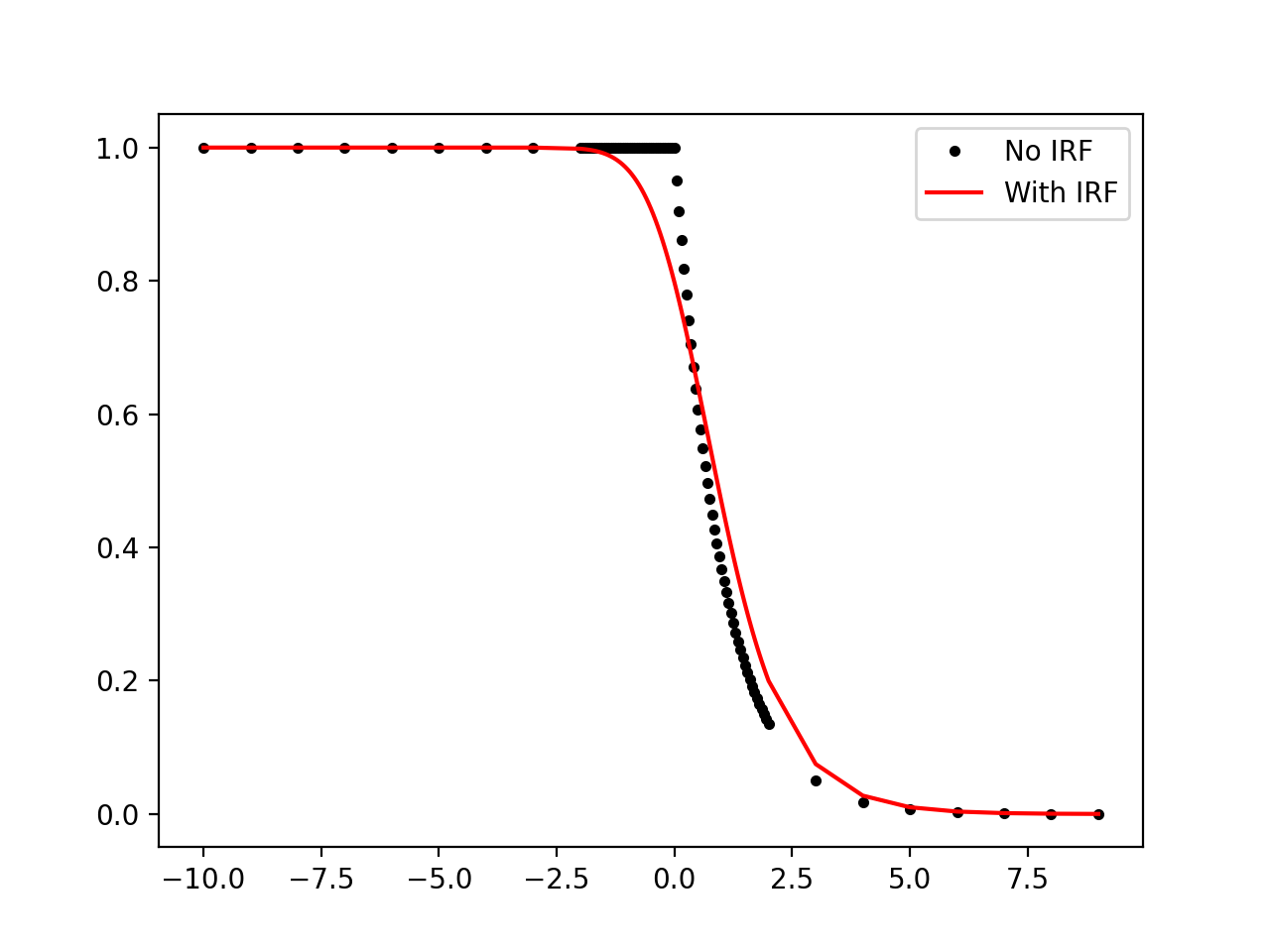
with_irf() also works with data that is not defined on an even grid, like many ultrafast experiments:
(Source code, png, hires.png, pdf)

Selections
In the context of ultrafast electron/x-ray scattering, time-series are assembled by selection a portion
of scattering patterns for each time-delay. The Selection class (and related subclasses) is
the generalization of selecting a rectangular area of scattering patterns to arbitrary patterns,
e.g. disks, torii, etc.
Instances can be used like boolean masks to select portions of scattering patterns. Consider an example where we want to know the integrated intensity in a Bragg peak:
>>> from skued import DiskSelection, diffread
>>>
>>> im = diffread(...)
>>>
>>> bragg = DiskSelection(shape = im.shape, center=(1024, 1024), radius=30)
>>> intensity = np.sum(im[bragg])
Selections really shine when trying to extract non-standard shapes, e.g. rings. You can use them in combination with iris-ued DiffractionDatasets to assemble specialized time-series.